COMP 100 Projects
Winter 2010
Pete Sanderson
Project 3 : Spreadsheet for monitoring workout heart
rates
Deadline: 11:59 pm Wednesday February 24 - credit reduced by 10% per day thereafter
20 points + 2 bonus point opportunity
The purpose of this assignment is to apply your knowledge of basic capabilities of Microsoft
Excel by building a spreadsheet for monitoring workout heart rates. This
is an individual assignment. You may receive help from your classmates but must
build the spreadsheet yourself.
Background: the Karvonen formula
The effectiveness of an aerobic training program can be measured by heart rate
during training using the Karvonen formula. According to the Karvonen formula,
a person's aerobic workout should be designed to maintain a heart rate within
a Training Zone.
- AGE is a person's age in years.
- RHR (Resting Heart Rate) is measured by the person's pulse at
rest, in beats per minute.
- MHR (Maximum Heart Rate) is calculated by: 220 - AGE
- The low end of the Training Zone is calculated by:
(MHR - RHR) * 0.50 + RHR
- The high end of the Training Zone is calculated by:
(MHR - RHR) * 0.85 + RHR
- Note that the "*" operator is multiplication.
Example: a 48 year old person with a Resting Heart Rate of 60.
AGE = 48
RHR = 60
MHR = 220 - AGE = 220 - 48 = 172
low end of Training Zone = (MHR - RHR) * 0.50 + RHR = (172 - 60) * 0.50 + 60 = 116
high end of Training Zone = (MHR - RHR) * 0.85 + RHR = (172 - 60) * 0.85 + 60 = 155
The training zone endpoints are rounded to the nearest whole number.
Overview of Your Assignment
You will transform a spreadsheet containing heart rate data into a useful tool
for tracking the effectiveness of an aerobic training program custom designed
for the Johnson family and based on the Karvonen formula.
David Johnson is 49 years old and has a resting heart rate of 74 beats per
minute.
His daughter Carol Johnson is 22 years old and has a resting heart rate of 58
beats per minute.
I have provided a "raw" spreadsheet called rawdata.xls with two named worksheets,
one for each member of the Johnson family. Each worksheet contains heart
rate measurements taken during four workouts.
- Rows 1 through 5 of each worksheet represent the elapsed time since the
start of the workout: 10, 20, 30, 40 and 50 minutes.
- Columns A, B, C, and D of each worksheet contains the five heart rate measurements for
the Tuesday, Thursday, Saturday, and Sunday workouts, respectively.
You must transform it, following the specifications below, into a spreadsheet
called heartrate.xls with two worksheets that resemble Figure 1 and one
that resembles Figure 2.
Important note: A spreadsheet which looks like this
can be generated by simply typing numbers and letters into the appropriate cells!
I will not give credit for such a solution. Most of the cells which display
numbers in fact contain formulas. Specifications for building the
spreadsheet are given below.
Important note: The images below contain
borders around certain cell boundaries. Your spreadsheet needs to include the
same borders. I have exaggerated the border thickness in these figures for clear
illustration; you may use the default thickness.
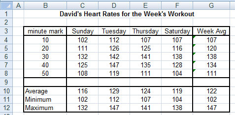
Figure 1. Resulting worksheet David. Format Carol's worksheet similarly.
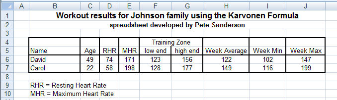
Figure 2. New worksheet called Summary
Detailed Specifications of Your Assignment
(point values shown in parentheses)
1. Start by downloading the Excel file rawdata.xls
(browse to this web page, right-click on the file name and select "Save Target As..." -- Firefox says Save Link As).
Save it in your home folder.
2. Open rawdata.xls using Excel. The instructions below are based on Excel 2007. If you need to use an older version, let me know.
3. Click the Office button, move to Prepare, and select Properties. For Title, type in "COMP 100 Project 3" (without the quotes).
For Subject, type "Johnson Workout Results" (without the quotes). For Author, replace my name with yours. Close the Properties. (1 point)
4. Save the file as heartrate (Excel automatically gives it .xls or .xlsx extension)
5. Transform worksheet David into its Figure 1 format by following
these instructions exactly:
-
Insert a blank column on the left by right-clicking on any cell
in column A, then selecting Insert and Entire Column. Insert another blank column on the left. Columns A and B should now
both be blank. In Column B, type in the values 10, 20, 30, 40 and 50 in rows 1 through 5 to represent the minute markers. (1 point)
-
Similarly insert 3 blank rows at the top. Then add labels as shown in rows 1 and 3 of Figure 1,
and labels as shown in cells B10, B11, and B12.
-
Center the row 1 title across columns B through G, using
Merge and Center
 (1
point)
(1
point)
-
Cell G4 will contain the average of the heart rates in
columns C through F of row 4. You must enter it as a function (

). Do the same for G5, G6, G7 and G8.
(1 point)
-
Row 10 cells: Cell C10 will contain the average of the five measurements
immediately above it in cells C4 through C8. You must enter it as a function.
Do the same for D10, E10, F10 and G10. (1 point)
-
Row 11 cells: Cell C11 will contain the minimum of the five measurements
above it in cells C4 through C8. Do the
same for D11, E11 and F11. Cell G11 will contain the minimum of the four minimums
C11, D11, E11 and F11. All cells must contain functions. (1 point)
-
Row 12 cells: Cell C12 will contain the maximum of the five measurements
above it in cells C4 through C8. Do the
same for D12, E12 and F12. Cell G12 will contain the maximum of the four maximums
C12, D12, E12 and F12. All cells must contain functions. (1 point)
-
Make sure all values display as whole numbers
(format cells for 0 decimal places), draw all cell borders as shown in Figure 1 (using

feature), and make sure cell contents are centered (except B10, B11, and B12).
(1 point)
6. Repeat Step 5 for the Carol worksheet.
7. Build a new worksheet called Summary as shown in Figure 2.
- Insert a new worksheet and rename it "Summary" (without the quotes), by
double-clicking the name. Reposition it so its tab appears to the
left of the other two. (1 point)
- Add titles and labels into the worksheet as shown in Figure 2. In the
subtitle, substitute your name for mine!
- Fill in Columns B, C and D. Fill in the Name, Age and
RHR columns as shown in Figure 2. These are all given. Columns
C and D contain the only numeric cells in this worksheet that are not formulas!
- Fill in Columns E, F and G. Enter mathematical formulas to calculate the
MHR, low end and high end of the training zone. (6 points)
- All formulas are given in the Background section at the top of the project.
- Remember that all formulas start with "="
- Format the cells so they are displayed as whole numbers.
- Except for the values 220, 0.50 and 0.85, all components of the formulas must be cell references!
- Here's how to test if you've done it
correctly: Change David's age to 55. The MHR should change to 165, the
low end should change to 120 and the high end to 151. If not, you're
doing it incorrectly. Don't forget to change his age back to 49.
- Fill in Column H. Cells H6 and H7 must refer to the average of averages
cell (G10) in the corresponding worksheet. (1 point)
- Fill in Column I. Cells I6 and I7 must refer to the "minimum of minimums"
cell (G11) in the corresponding worksheet. (1 point)
- Fill in Column J. Cells J6 and J7 must refer to the "maximum of maximums"
cell (G12) in the corresponding worksheet.
- Make sure all values display as whole numbers, draw all cell borders as shown in Figure 2 and center everything except Column B.
8. Create a chart of David's worksheet only and
place it right on the worksheet, as illustrated here. For full credit,
the chart needs to look exactly as shown in Figure 3, including the data lines
(1 point), the legend and title (1 point),
and the axis labels (1 point). You will need to use several
features in the Chart Tools Design tab and Layout tab to get the illustrated
results. If you are reading a printed copy of this project, view its web page on your browser for
a clearer color picture of the chart appearance.

Figure 3. Chart on David's worksheet
2 Point Bonus Option
For up to 2 points extra credit, format columns H and J in the
Summary worksheet to display their values in different colors using Excel's
Conditional Formatting feature. This feature must be used correctly as specified
below to get the credit.
- Columns H and J will utilize a feature called "conditional formatting".
To add "conditional formatting" to a cell, select it then choose Conditional
Formatting from the Styles group on the Home tab.
 From
here you can specify rules for setting the cell's text and background colors
depending on the value that the cell contains (or computes to). After you
select one of the conditions, Greater Than, Less Than, etc, a dialog box like
that shown in Figure 4 will appear.
From
here you can specify rules for setting the cell's text and background colors
depending on the value that the cell contains (or computes to). After you
select one of the conditions, Greater Than, Less Than, etc, a dialog box like
that shown in Figure 4 will appear.
- The conditional format for cells H6 and H7 (week average) is this:
if the week average is less than the Training Zone low end, display it as
"Yellow Fill with Dark Yellow Text". If between the Training Zone low
end and high end, display it as "Green Fill with Dark Green Text". If
above the Training Zone high end, display it as "Light Red Fill with Dark
Red Text". You need to use Conditional Formatting three times to do this.
Each condition/color combination is called a Rule. Figure 4 shows what to
specify for the first rule (week average less than Training Zone low end).
Note: You must provide a cell reference, as shown (1
point)
- The conditional format for cells J6 and J7 (week maximum) cells is this:
if the week maximum is above the MHR, display it as "Light Red Fill with Dark Red Text".
If less than MHR or equal to MHR, display it as "Green Fill with Dark Green Text". (1 point)
- The condition boundaries must be expressed using cell references, not
numeric values, to receive credit. The conditions must also be expressed correctly. If you are uncertain then select
the cell, go to
Conditional Formatting and select "Manage Rules...", the last item in the list. This will display all conditional
formatting rules for that cell and you can adjust them.
- If you do this correctly, the number in cell H6 will display in yellow,
cells J6 and H7 in green, and J7 in red.

Figure 4. Conditional formatting for first rule of cell H6
To Submit
Email me your spreadsheet file heartrate as an attachment to a message
to psanderson@otterbein.edu.
[
Pete Sanderson
|
Math Sciences server
|
Math Sciences home page
|
Otterbein
]
Last updated:
Pete Sanderson (PSanderson@otterbein.edu)